Creating and Visualizing Distance Fields with DataFrame

Introduction

Distance fields are a powerful representation of spatial data that have applications in computer graphics, computational geometry, path planning, and scientific visualization. They define, for each point in a space, the minimum distance to a set of reference objects or points.

In this tutorial, we'll explore how to:

• Generate a set of random reference points
• Create a regular sampling grid
• Compute a distance field relative to the reference points
• Export the results to CSV files
• Visualize the distance field using Python and Matplotlib

We'll use the DataFrame library, which provides powerful tools for working with spatial data and creates an elegant pipeline for processing and visualization.

Understanding Distance Fields

A distance field is a scalar field that specifies the minimum distance from any point to the closest object in a set. For each location in space, the distance field stores the distance to the nearest object. This creates a smooth gradient of values that:

• Equals zero at the objects themselves
• Gradually increases as you move away from objects
• Creates "ridges" of equidistant points between objects

This representation is particularly useful because:

• It encodes spatial relationships efficiently
• It simplifies many geometric operations like collision detection
• It can be used to create smooth transitions and blends
• It enables efficient path planning by following the gradient

Project Overview

Our project consists of two main parts:

1. A C++ program using the DataFrame library to generate the distance field data
2. A Python script that visualizes the results using Matplotlib

Here's the workflow we'll follow:

1. Generate random reference points in a 2D space
2. Create a regular grid of sample points
3. Calculate the distance from each grid point to the nearest reference point
4. Export the grid points, reference points, and distances to CSV files
5. Visualize the distance field as a 2D color map and a 3D surface

Distance Field with Reference Points

Step 1: Generate Random Points

First, we'll generate a set of random reference points in a 2D space. These points will be the "objects" that our distance field will measure distance from.

// Generate random reference points (nb_pts, min, max)
Serie reference_points =
    random_uniform(10, Vector2{-1.0, -1.0}, Vector2{1.0, 1.0});

This code uses the random_uniform function from the DataFrame library to create 10 random 2D points within a square area from (-1,-1) to (1,1). The points are stored in a Serie<Vector2>, which is a collection of 2D vectors.

The random_uniform function provides a convenient way to generate random data for testing and simulation. The DataFrame library offers various random distributions, including:

• random_uniform: Uniform distribution (equal probability across the range)
• random_normal: Normal (Gaussian) distribution
• random_poisson: Poisson distribution
• random_bernoulli: Bernoulli distribution

Step 2: Create Regular Grid

Next, we'll create a regular grid of points where we'll sample the distance field. This grid will define the resolution of our visualization.

// Create a regular grid for sampling (nb_pts, center, dimensions)
auto grid_points =
    grid::cartesian::from_dims<2>({100, 100}, {0.0, 0.0}, {2.0, 2.0});

This code creates a 100×100 regular grid centered at (0,0) with dimensions 2×2. This means the grid spans from (-1,-1) to (1,1), matching the domain of our reference points.

The from_dims function is part of the grid::cartesian namespace in the DataFrame library. It provides a convenient way to create uniform grids for sampling and visualization. The template parameter <2> specifies that we're creating a 2D grid.

Step 3: Compute Distance Field

With our reference points and sampling grid, we can now compute the distance field. For each point in the grid, we'll calculate the minimum distance to any reference point.

// Compute distance field (at, ref)
auto distances = distance_field<2>(grid_points, reference_points);

The distance_field function calculates the Euclidean distance from each grid point to the nearest reference point. It returns a Serie<double> containing these distances, which can be used for visualization and further analysis.

The template parameter <2> specifies the dimensionality of the space. The same function can be used for 3D or higher-dimensional distance fields by changing this parameter.

Step 4: Export to CSV

To visualize our distance field, we'll export the data to CSV files. We'll create two files:

• grid_points.csv: Contains the grid points with their calculated distances
• reference_points.csv: Contains the reference points

// Export results to CSV
df::io::write_csv(grid_points, "grid_points.csv");

// Export reference points
df::io::write_csv(reference_points, "reference_points.csv");

These code snippets write the data to CSV files in a simple format:

• grid_points.csv has columns for x, y, and distance
• reference_points.csv has columns for x and y

Note that while the DataFrame library includes IO capabilities for CSV and other formats, we're using standard C++ file output here for simplicity.

Step 5: Visualize with Python

Finally, we'll use Python with Matplotlib to create visualizations of our distance field. We'll create both a 2D contour plot and a 3D surface plot.

import numpy as np
import pandas as pd
import matplotlib.pyplot as plt
from matplotlib.colors import LinearSegmentedColormap
import argparse
import sys

def main():
    # Parse command line arguments
    parser = argparse.ArgumentParser(description='Visualize distance field from grid and reference points')
    parser.add_argument('grid_file', help='CSV file containing grid points and distances')
    parser.add_argument('ref_file', help='CSV file containing reference points')
    parser.add_argument('--output', '-o', default='distance_field', help='Base name for output files (default: distance_field)')
    args = parser.parse_args()

    try:
        # Read the data
        grid_data = pd.read_csv(args.grid_file)
        ref_points = pd.read_csv(args.ref_file)
    except FileNotFoundError as e:
        print(f"Error: Could not find input file: {e.filename}")
        sys.exit(1)
    except pd.errors.EmptyDataError:
        print(f"Error: File is empty")
        sys.exit(1)
    except pd.errors.ParserError:
        print(f"Error: File is not in the expected CSV format")
        sys.exit(1)

    # Reshape the data into a grid
    n = int(np.sqrt(len(grid_data)))  # Assuming square grid
    X = grid_data['x'].values.reshape(n, n)
    Y = grid_data['y'].values.reshape(n, n)
    Z = grid_data['distance'].values.reshape(n, n)

    # Create custom colormap
    colors = ['yellow', 'blue', 'lightblue', 'white', 'yellow', 'orange', 'red']
    n_bins = 100
    cmap = LinearSegmentedColormap.from_list("custom", colors, N=n_bins)

    # Create the 2D plot
    plt.figure(figsize=(12, 10))

    # Plot the distance field
    plt.contourf(X, Y, Z, levels=50, cmap=cmap)
    plt.colorbar(label='Distance')

    # Plot the reference points
    plt.scatter(ref_points['x'], ref_points['y'], 
               color='black', marker='o', s=30, 
               label='Reference Points')

    plt.title('Distance Field with Reference Points')
    plt.xlabel('X')
    plt.ylabel('Y')
    plt.axis('equal')
    plt.legend()
    plt.grid(True)

    # Save the 2D plot
    plt.savefig(f'{args.output}_2d.png', dpi=300, bbox_inches='tight')
    plt.close()

    # Create a 3D surface plot
    fig = plt.figure(figsize=(12, 10))
    ax = fig.add_subplot(111, projection='3d')

    surf = ax.plot_surface(X, Y, Z, cmap=cmap)
    ax.scatter(ref_points['x'], ref_points['y'], 
              np.zeros_like(ref_points['x']), 
              color='black', marker='o', s=30)

    plt.colorbar(surf, label='Distance')
    ax.set_title('3D View of Distance Field')
    ax.set_xlabel('X')
    ax.set_ylabel('Y')
    ax.set_zlabel('Distance')

    # Save the 3D plot
    plt.savefig(f'{args.output}_3d.png', dpi=300, bbox_inches='tight')
    plt.close()

if __name__ == '__main__':
    main()

This Python script:

1. Takes the paths to our CSV files as command-line arguments
2. Reads the data using pandas
3. Reshapes the grid data into a 2D grid for visualization
4. Creates a custom colormap for better visualization
5. Generates a 2D contour plot with reference points
6. Generates a 3D surface plot with reference points
7. Saves both plots as high-resolution PNG files

To run the visualization, execute the following command:

python3 plot.py grid_points.csv reference_points.csv

Visualization Analysis

Let's analyze the visualization we've created:

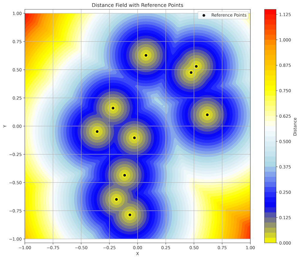
Distance Field with Reference Points

In this 2D visualization, we can observe several key features:

• Reference Points (Black Dots): These are the randomly generated points from which distances are measured.
• Yellow Centers: Areas immediately around reference points have distances approaching zero.
• Blue Regions: These represent areas with intermediate distances from reference points.
• Red/Orange Areas: Regions furthest from any reference point, typically in the corners of the domain.
• Contour Lines: Lines of equal distance that form concentric patterns around reference points.
• "Ridges": Blue regions between reference points where the distance function has local maxima.

The visualization clearly shows how the distance field creates a smooth gradient of values. The color transitions represent how the distance changes continuously throughout the space. The "ridges" between reference points are particularly interesting — they represent points that are equidistant from multiple reference points.

This type of visualization helps us understand the spatial relationship between points in our dataset and can reveal patterns that might not be obvious from the raw data.

Applications of Distance Fields

Distance fields have numerous applications across various domains:

Computer Graphics

• Font Rendering: Signed distance fields allow for high-quality text rendering at multiple scales.
• Ray Marching: Efficient rendering of complex 3D scenes using distance fields.
• Soft Shadows: Creating realistic soft shadows using distance information.

Computational Geometry

• Voronoi Diagrams: Distance fields are closely related to Voronoi diagrams.
• Medial Axis Extraction: Finding the "skeleton" of a shape using distance fields.
• Collision Detection: Quick proximity queries for game physics and simulations.

Path Planning

• Robot Navigation: Planning paths that maintain safe distances from obstacles.
• Potential Fields: Creating attractive/repulsive forces for agent navigation.
• Path Optimization: Finding smooth paths through complex environments.

Scientific Visualization

• Field Visualization: Representing electromagnetic, gravitational, or other fields.
• Isosurface Extraction: Identifying surfaces of equal value in volumetric data.
• Data Interpolation: Creating continuous representations from discrete samples.

Conclusion

In this tutorial, we've explored how to create and visualize distance fields using the DataFrame library and Python. We've seen how to:

• Generate random reference points in a 2D space
• Create a regular sampling grid
• Compute distances from grid points to reference points
• Export the data to CSV files
• Create visualizations of the distance field

Distance fields are a powerful representation for spatial data that can simplify many geometric operations and enable efficient algorithms for path planning, collision detection, and visualization. By combining the computational capabilities of the DataFrame library with the visualization power of Python and Matplotlib, we can create informative and visually appealing representations of complex spatial relationships.

The techniques we've explored can be extended to higher dimensions, different distance metrics, and more complex reference objects, making distance fields a versatile tool for a wide range of applications.